Free-slip Boundary Condition in CICE6 (AFIM / CICE_free-slip)

Last updated: 2026-01-15

This note documents the free-slip boundary condition implementation added to CICE6 in the AFIM/CICE_free-slip development branch, and how it interacts with the Lateral Drag Parameterisation (LDP) used to simulate Antarctic landfast ice.

---

Contents

1. Purpose and scope

2. Background: why free-slip matters

3. ice_in configuration

4. Code changes and control flow

5. Free-slip strain-rate discretisation

6. Interaction with Lateral Drag Parameterisation (LDP)

7. Deriving and interpreting C_s

8. Resolution dependence: why C_s can vary by 10–1000×

9. Mixed layer depth (hmix) in standalone-CICE

10. Practical tuning for the residual velocity u_0

11. Verification checklist

12. Caveats and known limitations

13. References

---

1. Purpose and scope

CICE historically behaves as no-slip along coastlines in many configurations, especially on a B-grid, because the velocity points adjacent to land are treated as inactive (or effectively pinned). This can:

• over-damp along-coast motion,

• over-stabilise coastal ice and promote unrealistically persistent “stuck” ice in channels, and

• contribute to excessive fast-ice build-up in some geometries.

The AFIM/CICE_free-slip branch adds a selectable free-slip option intended to:

• maintain no normal flow into land, while

• avoiding artificial suppression of tangential motion and shear at coastal boundaries,

• without changing the EVP rheology itself.

This implementation is designed for the C-grid momentum discretisation (grid_ice = "C" or "CD" variants), where normal/tangential components relative to a boundary can be represented more cleanly.

---

2. Background: why free-slip matters

2.1 Boundary conditions in CICE with C-grid-consistent velocity nomenclature

On the C-grid, the sea-ice velocity vector is represented on faces:

• E-faces (east/west faces): \((u_E, v_E)\), where \(u_E\) is the normal (x) component on the E-face and \(v_E\) is the tangential (y) component collocated on the same E-face.

• N-faces (north/south faces): \((u_N, v_N)\), where \(v_N\) is the normal (y) component on the N-face and \(u_N\) is the tangential (x) component collocated on the same N-face.

Let \(\mathbf{u}\) be the ice velocity and \(\mathbf{n}\) the outward unit normal to a boundary (with \(\mathbf{t}\) the unit tangent).

Continuous idealisations

• No-slip: $\( \mathbf{u}\cdot\mathbf{n} = 0 \quad \text{and} \quad \mathbf{u}\cdot\mathbf{t} = 0, \)$ i.e., both the normal and tangential components vanish at the boundary.

• Free-slip (idealised): $\( \mathbf{u}\cdot\mathbf{n} = 0 \quad \text{and} \quad \frac{\partial (\mathbf{u}\cdot\mathbf{t})}{\partial n} = 0, \)$ i.e., no penetration, but tangential flow is permitted with zero normal gradient (no imposed boundary-layer shear).

Mapping to C-grid face variables (grid-aligned walls)

For boundaries aligned with the grid, the normal/tangential components map directly onto the face velocities:

• Vertical wall (boundary normal in \(\pm x\)):

  • normal component: \(\mathbf{u}\cdot\mathbf{n} \leftrightarrow u_E\)

  • tangential component: \(\mathbf{u}\cdot\mathbf{t} \leftrightarrow v_E\)

• Horizontal wall (boundary normal in \(\pm y\)):

  • normal component: \(\mathbf{u}\cdot\mathbf{n} \leftrightarrow v_N\)

  • tangential component: \(\mathbf{u}\cdot\mathbf{t} \leftrightarrow u_N\)

Thus, a practical “C-grid” statement of the two boundary conditions is:

• No-slip (grid-aligned):

  • vertical wall: \(u_E = 0\) and \(v_E = 0\)

  • horizontal wall: \(v_N = 0\) and \(u_N = 0\)

• Free-slip (grid-aligned, idealised):

  • vertical wall: \(u_E = 0\) and \(\partial v_E/\partial x = 0\)

  • horizontal wall: \(v_N = 0\) and \(\partial u_N/\partial y = 0\)

Practical implementation in discrete EVP solvers (where it actually happens)

In EVP-type momentum solvers, the boundary condition is enforced primarily inside the strain-rate calculation, because strain rates require neighbour velocities to form finite differences. The numerical distinction is how “missing” neighbour values across land are treated when forming gradients of the tangential component:

• No-slip implementation (discrete)
  Missing neighbour values across land are effectively taken as zero (or the velocity point is masked out). This makes the tangential component drop to zero at the boundary and introduces large boundary shear consistent with a no-slip wall.

• Free-slip implementation (discrete)
  Missing neighbour values across land are replaced by a mirror / extrapolated value from the ocean side such that the tangential normal derivative is zero. Operationally, when a finite-difference stencil would reference a land-side neighbour, that neighbour is replaced by the adjacent ocean-side value (a “reflecting” or “zero-gradient” closure), so that $\( \frac{\partial v_E}{\partial x}\approx 0 \quad \text{at vertical walls}, \qquad \frac{\partial u_N}{\partial y}\approx 0 \quad \text{at horizontal walls}. \)$

This is why, in practice, “free-slip vs no-slip” in CICE is best understood as a strain-rate stencil choice (or ghost-value closure) rather than an explicit post-hoc modification of \((u_E,v_E,u_N,v_N)\) after the momentum step.

2.2 B-grid vs C-grid note

On a B-grid, the velocity point can sit in a way that makes coastline handling more “all-or-nothing” (velocity points can be deactivated when any corner of the cell is land), which behaves similarly to no-slip. On a C-grid, velocity components sit on faces, which better supports enforcing no-normal-flow while retaining tangential motion.

---

3. ice_in configuration

The free-slip behaviour is controlled through the namelist entry:

• boundary_condition = 'free_slip' (default remains no-slip unless specified)

In addition, if LDP is enabled, the following are relevant:

• coastal_drag = .true.

• Cs static coefficient, units \(m/s^2\)

• u0 residual speed, units \(m/s\)

• the form-factor configuration (F2 file and mapping method)

3.1 Example ice_in snippet

Below is a minimal excerpt consistent with the AFIM configuration (showing both free-slip and LDP):

&dynamics_nml
    boundary_condition    = 'free_slip'
    coastal_drag          = .true.
    Cs                   = 2e-3
    u0                   = 5e-4
/

&grid_nml
    F2_file           = '/path/to/form_factor_file.nc'
    F2x_varname       = 'F2x'
    F2y_varname       = 'F2y'
    F2_map_method     = 'max'     ! 'avg' or 'max'; default 'max'
    F2_test           = .false.
    F2_test_val       = 0.25
/

Notes

• boundary_condition is parsed as a string and used to set an internal logical noslip flag.

• F2_map_method controls how T-grid form factors are mapped onto velocity faces:

  • 'avg': average adjacent T-cell values to the face

  • 'max': take the maximum of adjacent values (more aggressive drag near rough coastlines)

---

4. Code changes and control flow

This section summarises where free-slip is applied and how it threads through the solver.

4.1 ice_dyn_evp.F90

Key additions/changes (AFIM/CICE_free-slip branch):

1. Initialisation
   In init_evp, after init_dyn_shared(dt_dyn), form factors are loaded when LDP is enabled:

   • if (coastal_drag) call load_F2_form_factors()

2. Boundary-condition selection A boundary_condition string is interpreted and a logical noslip is set, e.g.:

   • noslip = (trim(boundary_condition) == 'no_slip')

3. C-grid strain-rate call site In the C-grid EVP pathway, strain rates at the U-point are computed via either:

   • strain_rates_U_no_slip(...) (default CICE – no-slip)

   • strain_rates_U_free_slip(...) (new option – free-slip)

   depending on noslip.

4. LDP “Ku” update After stepu_C/stepv_C, the coastal stress factor is formed on E and N faces:

   • KuE = emass * F2E * Cs

   • KuN = nmass * F2N * Cs

   implemented via coastal_drag_stress_factor(...).

4.2 ice_grid.F90

A new routine load_F2_form_factors() reads pre-computed form factors from a NetCDF file and maps them onto:

• F2E (E-faces)

• F2N (N-faces)

Key behaviour:

• NaNs are converted to zero.

• A mapping from T-projection to faces is applied (avg or max).

• Values are scattered to blocks and halo-updated.

• A fallback test mode (F2_test) can apply uniform form factors on the domain perimeter.

4.3 ice_dyn_shared.F90

This module carries most of the free-slip implementation in practice:

• Defines the boundary_condition configuration variable.

• Implements strain_rates_U_free_slip(...).

• Adds LDP parameters/arrays (coastal_drag, Cs, u0, KuE/KuN, Kux/Kuy, etc.).

• Updates stepu_C and stepv_C to include a LDP contribution in the implicit momentum solve.

---

5. Free-slip strain-rate discretisation

5.1 Where free-slip is applied numerically

In this implementation, free-slip is enforced by how neighbour velocities are supplied to finite-difference gradients used in the U-point strain-rate calculation. The goal is to avoid forcing tangential components to zero solely because the adjacent point lies on land.

The free-slip routine uses the existing edge masks:

• epm — E-face activity mask

• npm — N-face activity mask

These are typically 1 for active ocean/ice velocity points and 0 for land/inactive.

5.2 Reflection-style neighbour substitution (key idea)

When a neighbour velocity lies across land (mask = 0), the free-slip formulation replaces it with a reflected/copy value from the interior side, e.g. schematically:

• If epm(i,j) = 1 but epm(i,j+1) = 0 (north neighbour is land), then
  use vvelE(i,j) as the “north neighbour” when forming \(\partial v/\partial y\).

This is implemented by blending masked neighbours, for example (illustrative form):

\[ v^{E}_{i,j+1} \leftarrow v^{E}_{i,j+1}\,epm_{i,j+1} + (epm_{i,j}-epm_{i,j+1})\,epm_{i,j}\,v^{E}_{i,j} \]

which reduces to:

• \(v^{E}_{i,j+1}\) when epm(i,j+1)=1, and

• \(v^{E}_{i,j}\) when epm(i,j+1)=0 and epm(i,j)=1.

Analogous substitutions are performed for the other neighbour directions/components needed by the U-point strain-rate operator.

5.3 Effect on the strain-rate tensor

Using interior-value substitution across land effectively enforces:

• no normal flow at land boundaries (through the underlying masks/velocity placement), and

• zero normal gradient of tangential velocity in the discrete derivative (free-slip analogue)

rather than forcing the tangential component itself to zero.

---

6. Interaction with Lateral Drag Parameterisation (LDP)

Free-slip and LDP address different physical/numerical issues:

• Free-slip relaxes artificial tangential pinning imposed by boundary handling.

• LDP adds an explicit lateral momentum sink tied to coastline roughness and ice mass.

In AFIM/CICE_free-slip, these can be used together: free-slip provides the numerically permissive boundary, while LDP supplies the physically motivated coastal damping needed to sustain realistic landfast ice.

6.1 LDP stress law (from Liu et al. 2022)

The lateral (coastal) drag stress is written as (one of the Liu et al. variants):

\[ \boldsymbol{\tau}_{\ell} = m\,F_2\,C_s\,\frac{\mathbf{u}}{\lvert\mathbf{u}\rvert + u_0} \]

where:

• \(m\) is sea-ice mass per unit area (kg/m\(^2\)), typically \(m = \rho_i\,h\,a\)

• \(F_2\) is a dimensionless form factor representing effective coastline roughness/orientation

• \(C_s\) is a tunable coefficient with units of acceleration (m/s\(^2\))

• \(u_0\) is a small residual speed (m/s) preventing a singularity as \(|u|\to 0\)

This formulation transitions between:

• linear drag at very small speeds (regularised by \(u_0\)), and

• a capped (approximately constant-magnitude) stress as \(|u|\gg u_0\).

6.2 How LDP enters the C-grid momentum solve

Implementation pattern:

1. Compute a stress scale on faces:

   \[ K_u = m\,F_2\,C_s \]

   where m is taken as emass or nmass (face mass per area).

2. Convert to an implicit drag coefficient:

   \[ C_\ell = \frac{K_u}{\lvert\mathbf{u}\rvert + u_0} \]

   (units kg m\(^2 s\)^{-1}$).

3. Add \(C_\ell\) into the implicit coefficient cca in stepu_C/stepv_C.

4. Export diagnostic stress components:

   • \(\mathrm{Kux} = -u * C_{\ell}\)

   • \(\mathrm{Kuy} = -v * C_{\ell}\)

These outputs are useful for confirming where and how strongly LDP is acting.

---

7. Deriving and interpreting \(C_s\)

In AFIM’s CICE coastal (lateral) drag implementation, the stress scale is set by the product of:

• an ice mass per unit area \(m\) (kg m\(^{-2}\)),

• a dimensionless form factor \(F_2\) (unitless), and

• a tunable coefficient \(C_s\) (m s\(^{-2}\)),

via:

\[ K_u = m\,F_2\,C_s, \]

where \(K_u\) has units of stress (Pa). In the momentum solve, this stress scale is applied in a velocity-dependent way via the regularisation speed \(u_0\) (see the “Practical note” below).

7.1 Units and physical meaning

From

\[ K_u = m\,F_2\,C_s, \]

• \(m\) has units kg m\(^{-2}\)

• \(F_2\) is dimensionless

• \(C_s\) has units m s\(^{-2}\)

Therefore:

\[ [K_u] = \mathrm{kg\,m^{-2}}\cdot 1 \cdot \mathrm{m\,s^{-2}} = \mathrm{kg\,m^{-1}\,s^{-2}} = \mathrm{N\,m^{-2}} = \mathrm{Pa}. \]

So \(C_s\) is an acceleration scale. A useful interpretation is:

\(C_s\) sets the maximum lateral-drag deceleration per unit ice mass in a cell with \(F_2=1\), expressed as an equivalent stress scale \(K_u\) (Pa).

A back-of-envelope conversion is:

• \(C_s = 10^{-4}\,\mathrm{m\,s^{-2}}\) corresponds to a speed change of

  \[ \Delta u \approx C_s\,\Delta t \approx 10^{-4}\times 86400 \approx 8.6\times10^{-3}\ \mathrm{m\,s^{-1}} \]

  per day.

7.2 Stress magnitude relative to wind stress

Representative (“nominal”) ice properties:

• \(\rho_i \approx 900\,\mathrm{kg\,m^{-3}}\),

• \(h_i \approx 1\,\mathrm{m}\), so the column ice mass per unit area is:

\[ m \approx \rho_i h_i \approx 900\,\mathrm{kg\,m^{-2}}. \]

Then, for \(C_s=10^{-4}\,\mathrm{m\,s^{-2}}\),

\[ m\,C_s \approx 900\times10^{-4} = 0.09\ \mathrm{Pa}. \]

If \(F_2\approx 1\), this implies \(K_u\approx 0.09\) Pa, comparable to typical Antarctic wind-stress magnitudes (\(\mathcal{O}(0.1)\) Pa). This is broadly consistent with the motivation in Liu et al. (2022), where the lateral-drag stress scale is intended to be dynamically competitive with atmospheric and ocean stresses in near-coastal fast-ice regimes.

7.3 A practical \(C_s\) tuning rule (given a target stress scale)

If we have a target peak lateral stress magnitude \(\tau^{\ast}\) (Pa) for a representative coastal cell, then:

\[ C_s(\tau^{\ast},F_2) \approx \frac{\tau^{\ast}}{m\,F_2}. \]

Example:

• \(\tau^{\ast} = 10\ \mathrm{Pa}\),

• \(m = 900\ \mathrm{kg\,m^{-2}}\),

• \(F_2=1\),

gives:

\[ C_s \approx \frac{10}{900\times 1} \approx 1.1\times 10^{-2}\ \mathrm{m\,s^{-2}}. \]

This sits within the AFIM test range (\(10^{-4}\)–\(10^{-2}\)), but the effective value depends strongly on local \(F_2\).

---

7.4 Parameter-space view: \(C_s(\tau^{\ast},F_2)\)

The figure below visualises the tuning rule

\[ C_s(\tau^{\ast},F_2)=\frac{\tau^{\ast}}{m\,F_2} \]

over a log–log range \(\tau^{\ast}\in[0.1,100]\) Pa and \(F_2\in[0.1,100]\) using \(m=900\) kg m\(^{-2}\).

Key takeaways:

• Increasing \(\tau^{\ast}\) (moving right) requires larger \(C_s\).

• Increasing \(F_2\) (moving up) allows smaller \(C_s\) for the same \(\tau^{\ast}\).

• Contours are lines of constant \(\tau^{\ast}/F_2\) (i.e., constant \(C_s\) for fixed \(m\)).

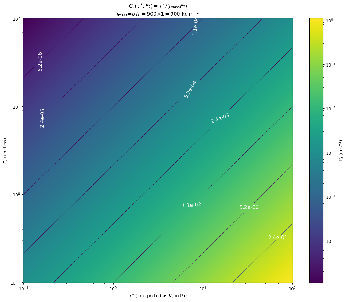
Parameter-space plot of \(C_s(\tau^{\ast},F_2)=\tau^{\ast}/(mF_2)\) for \(m=\rho_i h_i=900\times 1 = 900\) kg m\(^{-2}\). Color shows \(C_s\) (m s\(^{-2}\)); contours are log-spaced \(C_s\) levels.

Practical usage: a plausible \(\tau^{\ast}\) (what peak lateral stress is rational given the model’s physical-scheme to be capable of), then read off the implied \(C_s\) over the range of \(F_2\) values actually present on the grid (coastline- and GI-dependent).

---

7.5 Companion view: the implied stress scale \(K_u(C_s,F_2)\)

In CICE lateral drag is numerically implemented first by computing

\[ K_u(C_s,F_2)=mF_2C_s, \]

which makes it somewhat potentially easier to think of in terms of the actual stress scale \(K_u\) (Pa) implied by a chosen \(C_s\) and the spatially varying \(F_2\) field.

Some important points:

• At fixed \(C_s\), larger \(F_2\) produces larger \(K_u\).

• At fixed \(F_2\), increasing \(C_s\) scales \(K_u\) linearly.

• This plot is the “inverse” of the previous one and is useful for sanity-checking what stress magnitudes for a chosen \(C_s\) will imply across the domain.

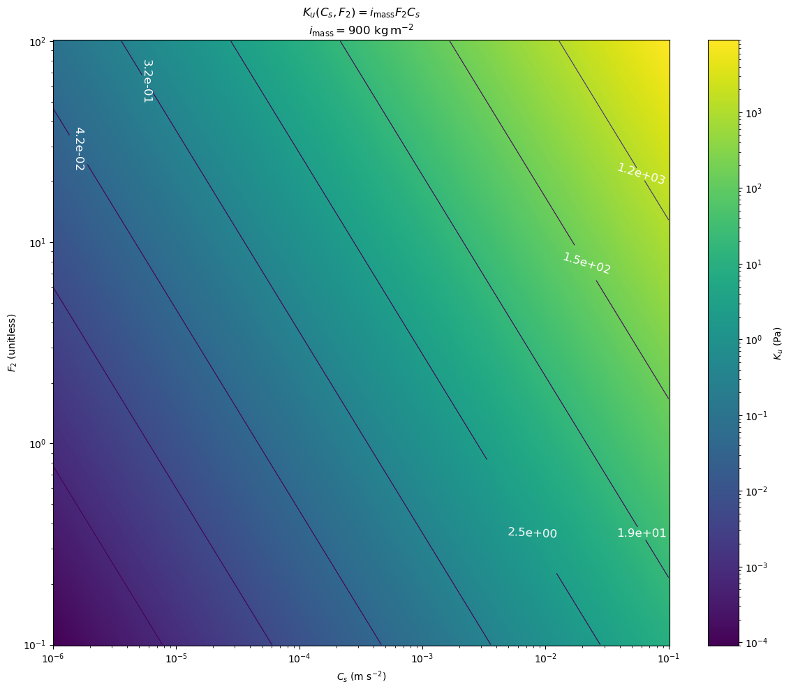
Companion parameter-space plot of \(K_u(C_s,F_2)=mF_2C_s\) (Pa), using \(m=900\) kg m\(^{-2}\). Color shows \(K_u\); contours are log-spaced \(K_u\) levels. This is useful for interpreting a chosen \(C_s\) in terms of the implied coastal stress scale across the local \(F_2\) distribution.

---

7.6 Practical note: why \(\tau^{\ast}\) is a “maximum stress” in the solver (role of \(u_0\))

In the C-grid momentum solve, the lateral-drag contribution is implemented using a speed scale:

\[ c = |\mathbf{u}| + u_0, \qquad C_l = \frac{K_u}{c}, \qquad \boldsymbol{\tau}_{\mathrm{coast}} \sim -\,C_l\,\mathbf{u}. \]

This implies a stress magnitude scaling like:

\[ |\boldsymbol{\tau}_{\mathrm{coast}}| \sim \frac{K_u\,|\mathbf{u}|}{|\mathbf{u}|+u_0}. \]

So:

• for \(|\mathbf{u}|\gg u_0\), the stress asymptotes to \(|\boldsymbol{\tau}_{\mathrm{coast}}|\to K_u\) (i.e., \(K_u\) behaves like a maximum stress scale);

• for \(|\mathbf{u}|\ll u_0\), the stress becomes small and approximately linear in speed, \(|\boldsymbol{\tau}_{\mathrm{coast}}|\approx K_u\,|\mathbf{u}|/u_0\).

This is one reason it is meaningful to treat \(\tau^{\ast}\) as a “target peak stress” when using this “tuning rule”

\[ C_s \approx \frac{\tau^{\ast}}{mF_2}. \]

---

8. Resolution dependence and tuning behaviour: why \(C_s\) can vary by 10–1000×

8.0 What we observed in AFIM (1993 example)

In the AFIM CICE6 Antarctic configuration, increasing the lateral-drag coefficient \(C_s\) produces a strong, increase in pan-Antarctic fast-ice area (FIA), while leaving pan-Antarctic sea-ice area (SIA) essentially unchanged over the same year. In other words, \(C_s\) primarily controls the partitioning of coastal ice into “immobile” versus “mobile” regimes (through the momentum balance), rather than materially altering the basin-scale thermodynamic ice edge that dominates SIA.

At the same time, fast-ice thickness (FIT) and mean sea-ice thickness (SIT) can exhibit a measurable response to \(C_s\):

• FIT responds because changing \(C_s\) changes (i) the extent of the fast-ice mask and (ii) the mechanical redistribution within the coastal zone; a larger fast-ice mask can also lower the area-mean FIT if it expands into thinner, newly-classified regions.

• SIT is typically much less sensitive in these tests, consistent with SIA invariance and the fact that most of the pack-ice thermodynamic budget is not directly targeted by lateral drag.

8.1 Some thoughts on why FIA is sensitive to \(C_s\) but SIA is not

Coastal drag enters the momentum equation as an additional sink proportional to velocity (implemented as a stress term that is strongest where the form factor \(F_2\) is non-zero). This tends to:

1. reduce coastal ice speeds and shear along the land/ice boundary,

2. increase the persistence of near-coastal immobility, and therefore

3. expand the diagnosed landfast-ice mask and FIA.

However, SIA is primarily set by the large-scale balance of surface fluxes and the thermodynamic ice edge over the open Southern Ocean. Because lateral drag is geographically confined to a comparatively small fraction of the domain and acts primarily on dynamics (not directly on thermodynamic freezing potential), its integrated impact on basin-scale SIA can be weak—consistent with the near-overlap of SIA curves across \(C_s\) in 1993.

8.2 Area-averaging a line (or narrow-strip) momentum sink

Lateral drag originates from interactions along (or very near) a boundary—effectively a line or narrow strip process. Models apply momentum tendencies as area-averaged stresses over grid cells. If the effective coastal boundary layer has physical width \(w\) (km), but the grid spacing is \(\Delta\) (km), then the fraction of a coastal cell that “should feel” boundary drag is roughly

\[ f \sim \frac{w}{\Delta}. \]

If the scheme applies drag over the whole cell (or an entire face/control area), maintaining the same integrated momentum sink suggests compensating the area-mean stress by approximately \(1/f \sim \Delta/w\). Since (to leading order) \(\tau \propto C_s\), this implies a heuristic scaling

\[ C_s(\Delta) \propto \frac{\Delta}{w}. \]

8.3 Sub-grid coastline complexity (partly handled by \(F_2\))

The form factor \(F_2\) is designed to represent unresolved coastline roughness/orientation within a cell. When \(F_2\) is computed from high-resolution coastline and grounded-iceberg geometry, it can partially compensate for resolution effects by increasing effective drag where sub-grid boundary complexity is high.

Nevertheless, \(F_2\) cannot remove resolution dependence entirely because:

• drag still enters as an area-mean stress (and the relevant area increases with \(\Delta\)),

• landfast physics depends on narrow anchored features that may not exist at coarse resolution, and

• the effective width \(w\) of the coastal shear/anchor zone is not universal (it depends on coastline geometry, grounded-iceberg pinning, and the local stress regime).

8.4 Worked scaling examples (orders-of-magnitude)

Assume \(w = 5\,\mathrm{km}\) for an effective coastal anchor/shear zone. Then:

Grid spacing \(\Delta\)	\(\Delta/w\)	Implication for \(C_s\)
5-50 km	0.001-1	baseline tuning (e.g., order \(10^{-4}\)–\(10^{-2}\) m s\(^{-2}\))
50-100 km	1-10	order-of-magnitude larger \(C_s\) may be needed
100-500 km	10-100	two orders of magnitude larger \(C_s\) may be needed

If instead \(w\sim 0.5\,\mathrm{km}\) (e.g., narrow fjords or strong grounded-iceberg pinning), then:

• 50 km grid: \(\Delta/w\sim 100\)

• 500 km grid: \(\Delta/w\sim 1000\)

This provides a practical rationale for the 10–1000× tuning envelope encountered across model resolutions and regions. In AFIM, because \(F_2\) is computed from high-resolution coastline/GI geometry, some of this scaling may be moderated; the table should be treated as a tuning heuristic, not a strict rule.

8.5 Example figures (1993) showing \(C_s\) sensitivity in FIA but not SIA

The following time series illustrate the key empirical behaviour used to guide tuning: FIA increases strongly with \(C_s\), while pan-Antarctic SIA remains nearly unchanged over the same year. FIT and SIT provide additional context on thickness responses.

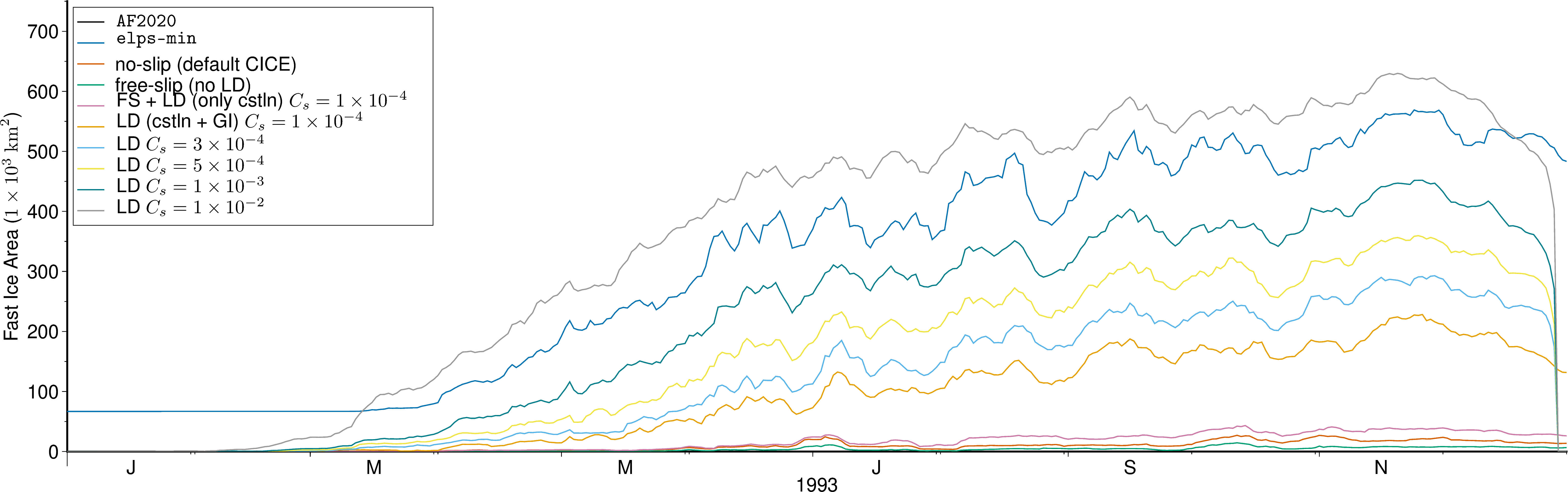
Pan-Antarctic fast-ice area (FIA) in 1993 across a sweep of \(C_s\). Increasing \(C_s\) yields a strong increase in FIA, consistent with stronger lateral drag promoting fast-ice persistence and extent in coastline/GI-adjacent regions.

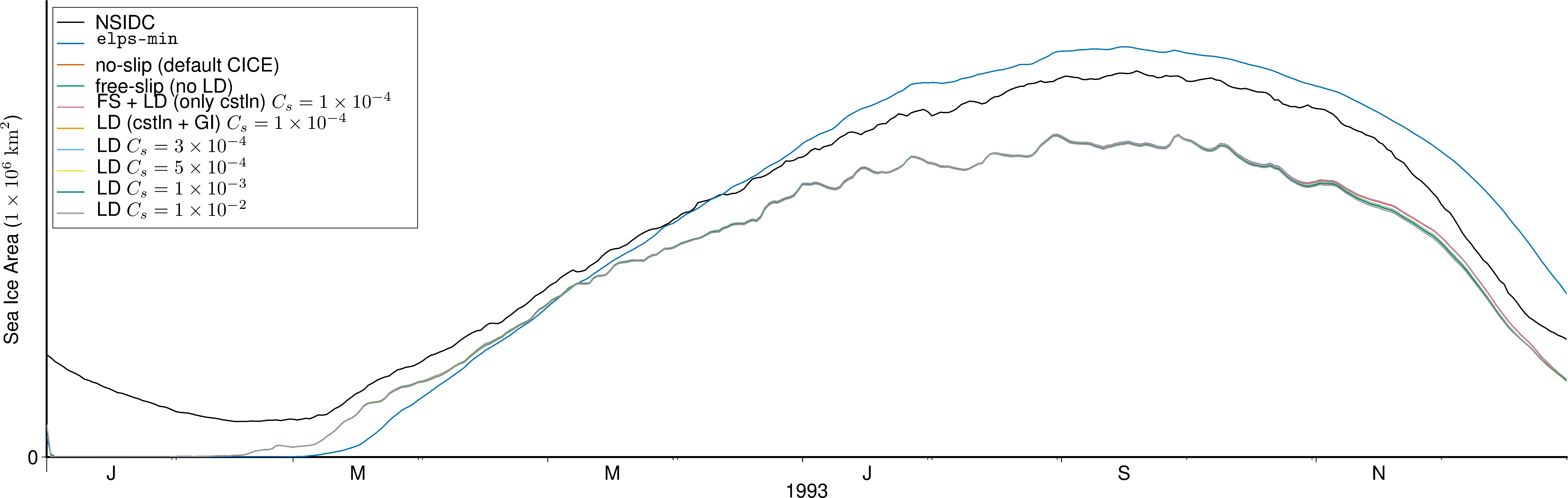
Pan-Antarctic sea-ice area (SIA) in 1993 across the same \(C_s\) sweep. In this experiment set, SIA is largely insensitive to \(C_s\) (curves overlap closely), indicating that tuning \(C_s\) can target fast-ice behaviour without materially degrading basin-scale SIA.

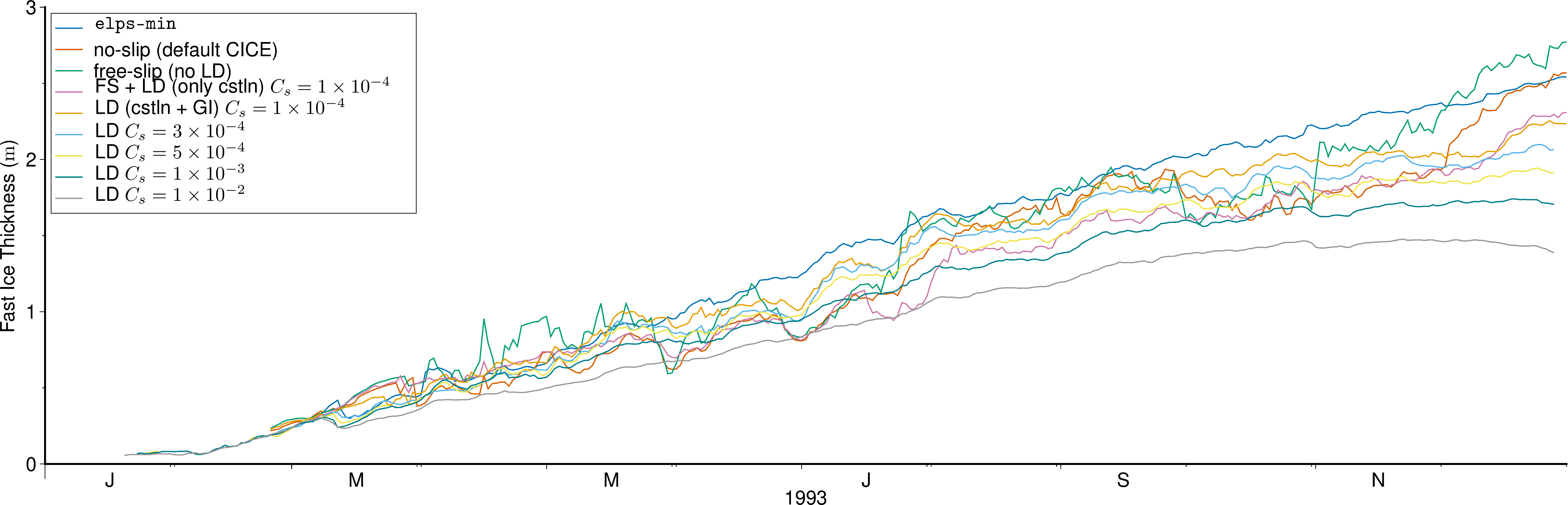
Fast-ice thickness (FIT) in 1993 across the \(C_s\) sweep. Thickness responds to \(C_s\), reflecting redistribution of fast ice across a changing fast-ice mask and changes in the dynamical/thermodynamic balance under stronger lateral drag.

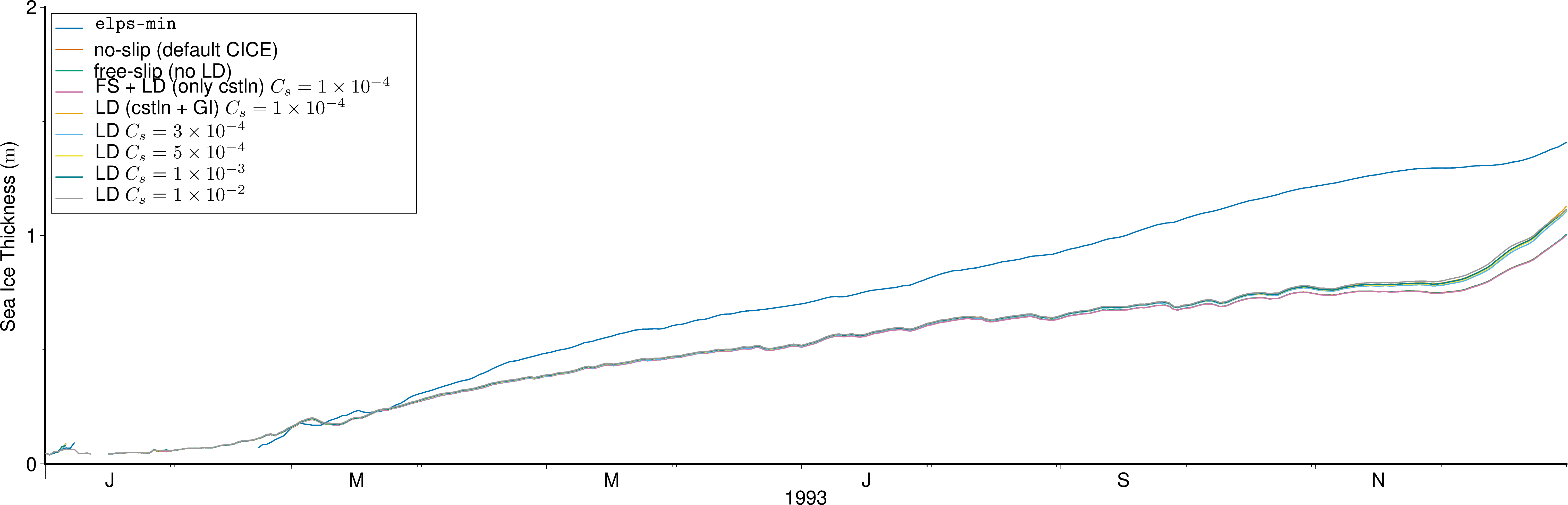
Sea-ice thickness (SIT) in 1993 across the \(C_s\) sweep. SIT exhibits comparatively weaker sensitivity than FIT in this experiment set, consistent with \(C_s\) primarily acting in coastline/GI-adjacent cells rather than over the broader pack.

---

9. Mixed-layer depth in standalone CICE

In standalone (uncoupled) CICE/Icepack runs, the ocean mixed layer is represented as a single-layer slab with finite heat capacity. The prognostic sea-surface temperature (sst) is updated from the net surface and basal heat fluxes, and the mixed-layer depth hmix (m) sets the effective heat capacity per unit area. Consequently, for a given net heat flux, SST tendencies scale approximately as \(1/h_\mathrm{mix}\).

9.1 Mixed-layer energy balance implemented in Icepack

The mixed-layer update used in icepack_ocn_mixed_layer can be summarised by decomposing the contributing flux terms.

(i) Absorbed shortwave at the ocean surface

The absorbed shortwave flux is

\[ \mathrm{swabs} = (1-\alpha_{\mathrm{v,dir}})\,\mathrm{swvdr} + (1-\alpha_{\mathrm{ir,dir}})\,\mathrm{swidr} + (1-\alpha_{\mathrm{v,dif}})\,\mathrm{swvdf} + (1-\alpha_{\mathrm{ir,dif}})\,\mathrm{swidf}, \]

where the \(\alpha\)’s are spectral-band ocean albedos (fractions), and sw* are downwelling shortwave components (W m\(^{-2}\)).

(ii) Outgoing longwave

With \(T_\mathrm{sfK}=\mathrm{sst}+T_\mathrm{ffresh}\) (Kelvin),

\[ \mathrm{flwout\_ocn} = -\sigma T_\mathrm{sfK}^4, \]

where \(\sigma\) is the Stefan–Boltzmann constant.

(iii) Sensible and latent turbulent fluxes (bulk-aero form)

Given transfer coefficients shcoef and lhcoef,

\[ \mathrm{fsens\_ocn} = \mathrm{shcoef}\,\Delta T, \qquad \mathrm{flat\_ocn} = \mathrm{lhcoef}\,\Delta q, \qquad \mathrm{evap\_ocn} = -\frac{\mathrm{flat\_ocn}}{L_\mathrm{vap}}. \]

(iv) Prognostic SST tendency (primary dependence on hmix)

Let \(c_p\rho\) be the seawater volumetric heat capacity (J m\(^{-3}\) K\(^{-1}\)), and \(\Delta t\) the time step. Icepack updates SST as

\[ \mathrm{sst} \leftarrow \mathrm{sst} + \frac{\Delta t}{c_p\rho\,h_\mathrm{mix}} \Big[ (\mathrm{fsens\_ocn}+\mathrm{flat\_ocn}+\mathrm{flwout\_ocn}+\mathrm{flw}+\mathrm{swabs}) (1-a_\mathrm{ice}) +(\mathrm{fhocn}+\mathrm{fswthru}) \Big]. \]

The open-water atmospheric exchange term is multiplied by \((1-a_\mathrm{ice})\), so its influence diminishes as ice concentration approaches unity. The key implication is immediate:

For a given net cooling/heating (W m\(^{-2}\)), the SST response magnitude scales like \(1/h_\mathrm{mix}\).

(v) Deep-ocean heat flux adjustment

A prescribed “deep ocean” heat flux term qdp (W m\(^{-2}\)) further modifies SST:

\[ \mathrm{sst} \leftarrow \mathrm{sst} - \frac{\mathrm{qdp}\,\Delta t}{c_p\rho\,h_\mathrm{mix}}. \]

(vi) Freezing/melting potential passed to thermodynamics

Icepack computes the freezing/melting potential (W m\(^{-2}\)) as

\[ \mathrm{frzmlt} = \frac{(T_f-\mathrm{sst})\,c_p\rho\,h_\mathrm{mix}}{\Delta t}, \qquad \mathrm{frzmlt} \in [-1000,\,1000], \]

and if \(\mathrm{sst}\le T_f\) it resets \(\mathrm{sst}\leftarrow T_f\).

A useful consequence is that once SST is routinely being driven to \(T_f\) each step (i.e., the mixed layer is “pinned” at freezing), \(\mathrm{frzmlt}\) tends to reflect the net cooling flux required to maintain \(T_f\) rather than strongly reflecting \(h_\mathrm{mix}\). This helps explain why wintertime growth rates and the timing of the seasonal maximum can be relatively insensitive to hmix in heavily ice-covered conditions.

(vii) Diagnostic freeze-up timescale

If the mixed layer must cool by \(\Delta T\) under a representative net cooling magnitude \(|Q|\) (W m\(^{-2}\)), then a characteristic cooling time is

\[ t_\mathrm{cool} \sim \frac{c_p\rho\,h_\mathrm{mix}\,\Delta T}{|Q|}, \]

so, absent strong restoring, freeze-up timing shifts approximately linearly with \(h_\mathrm{mix}\).

9.2 Practical conceptual model for Southern Ocean SIA sensitivity to hmix

We cannot deduce an exact numerical Southern Ocean sea-ice area (SIA) time series from hmix alone because SIA depends on the imposed forcing, initial SST, the ice–ocean heat flux terms (fhocn, fswthru, qdp), and the evolving ice concentration aice. However, the slab-ocean equations above allow a robust deduction of the direction, seasonal phasing, and a useful scaling for how changing hmix affects SIA in standalone CICE/Icepack.

(i) What hmix controls

The mixed-layer depth enters as thermal inertia through the mixed-layer heat capacity:

\[ \Delta \mathrm{sst} \propto \frac{\Delta t}{c_p\rho\, h_\mathrm{mix}}\;(\text{net heat flux}). \]

Collapsing the terms in the SST update gives the schematic form

\[ \mathrm{sst}_{n+1}=\mathrm{sst}_n + \frac{\Delta t}{c_p\rho\, h_{\mathrm{mix}}}\Big[(Q_{\mathrm{atm}})(1-a_{\mathrm{ice}}) + Q_{\mathrm{ice\to ocn}}\Big] - \frac{\Delta t}{c_p\rho\, h_{\mathrm{mix}}}q_{dp}, \]

where

• \(Q_{\mathrm{atm}} = f_{\mathrm{sens}}+f_{\mathrm{lat}}+f_{\mathrm{lw,out}}+f_{\mathrm{lw,in}}+f_{\mathrm{sw,abs}}\),

• \(Q_{\mathrm{ice\to ocn}}=f_{hocn}+f_{swthru}\).

Holding fluxes fixed:

• smaller hmix (e.g., 10 m) \(\rightarrow\) SST responds faster to surface fluxes,

• larger hmix (e.g., 60 m) \(\rightarrow\) SST responds slower (greater inertia).

The freezing/melting potential is

\[ \mathrm{frzmlt}=\frac{(T_f-\mathrm{sst})\,c_p\rho\,h_{\mathrm{mix}}}{\Delta t}, \]

with \(\mathrm{sst}\) reset to \(T_f\) whenever \(\mathrm{sst}\le T_f\). Therefore, the timing of reaching \(T_f\) over open water is the aspect most directly controlled by hmix.

(ii) A simple scaling for autumn cooling

Take a representative autumn net cooling over open water of \(Q_{\mathrm{net}}=-100\ \mathrm{W\,m^{-2}}\) and \(\Delta t=86400\ \mathrm{s}\) (daily). With \(c_p\rho\approx 4.1\times10^6\ \mathrm{J\,m^{-3}\,K^{-1}}\),

\[ \Delta T_{\text{day}} \approx \frac{Q_{\text{net}}\Delta t}{c_p\rho\, h_{\mathrm{mix}}}. \]

This yields:

• 10 m: \(\Delta T_{\text{day}} \approx -0.21\ \mathrm{K\,day^{-1}}\)

• 20 m: \(\approx -0.105\ \mathrm{K\,day^{-1}}\)

• 60 m: \(\approx -0.035\ \mathrm{K\,day^{-1}}\)

Time to cool by 1 K under this flux:

• 10 m: \(\sim\)4.8 days

• 20 m: \(\sim\)9.5 days

• 60 m: \(\sim\)28.6 days

Thus, if large open-water areas are typically 1–2 K above freezing during autumn, increasing hmix from 20 m to 60 m can plausibly delay widespread attainment of \(T_f\) by weeks, delaying freeze-up and suppressing early-season areal growth.

(iii) Expected seasonal ordering of Southern Ocean SIA

Because Antarctic SIA is strongly shaped by freeze-up timing, winter expansion, and spring retreat, the dominant effect of increasing hmix is typically a damping and phase lag of the seasonal cycle.

Autumn / early winter (advance):

\[ \mathrm{SIA}_{10m} > \mathrm{SIA}_{20m} > \mathrm{SIA}_{60m}. \]

A shallower mixed layer cools to \(T_f\) sooner over open water, enabling earlier ice formation and faster areal advance.

Mid-winter peak (maximum SIA):

\[ \mathrm{SIA}^{\max}_{10m} \gtrsim \mathrm{SIA}^{\max}_{20m} \gtrsim \mathrm{SIA}^{\max}_{60m}, \]

but differences often shrink once SST is pinned near \(T_f\) under extensive ice and the atmospheric term is suppressed by \((1-a_{\mathrm{ice}})\).

Spring / early summer (retreat): Late in the season the ordering can partially reverse:

\[ \mathrm{SIA}_{60m} \gtrsim \mathrm{SIA}_{20m} \gtrsim \mathrm{SIA}_{10m}, \]

because a deeper mixed layer warms more slowly above freezing, potentially delaying melt and retreat.

(iv) Annual-mean SIA

Annual-mean SIA may change less than the seasonal phasing because:

• shallower hmix tends to increase winter SIA but can accelerate summer retreat, and

• deeper hmix tends to delay advance but can delay retreat.

A concise qualitative summary is therefore:

• 10 m: earlier advance, larger early-winter SIA, potentially slightly larger maximum, earlier retreat.

• 60 m: delayed advance (potentially by weeks), smaller early-winter SIA and possibly smaller maximum, later retreat.

• 20 m: intermediate.

(v) Important nuance: “standalone” still has local coupling

Even in standalone mode there remains an ice–slab-ocean coupling: aice feeds back on SST via the \((1-a_{\mathrm{ice}})\) factor on atmospheric fluxes and via the ice-to-ocean terms (fhocn, fswthru). What is absent is a dynamically responding ocean circulation and associated lateral heat transport; hmix therefore controls local slab heat capacity, not ocean heat convergence.

---

10. Practical tuning for the residual velocity

In AFIM’s lateral drag implementation, the residual velocity \(u_0\) enters the momentum update through the speed-dependent drag coefficient used for both seabed stress and coastal drag. In the C-grid LDP code (e.g., stepu_C, stepv_C) the relevant definitions are:

• Ice speed: \(|\mathbf{u}| = \sqrt{u^2 + v^2}\)

• Regularised speed: \(|\mathbf{u}| + u_0\)

• Coastal drag “coefficient” (in the solver denominator):

  \[ C_\ell = \frac{K_u}{|\mathbf{u}| + u_0} \]

• Coastal drag stress (vector form; schematically):

  \[ \boldsymbol{\tau}_{\mathrm{LDP}} \propto -\,C_\ell\,\mathbf{u} = -\,\frac{K_u}{|\mathbf{u}| + u_0}\,\mathbf{u}. \]

Here \(K_u\) is the (precomputed) lateral-drag stress scale (KuE, KuN) and is proportional to \(C_s\) via

\[ K_u \propto F_2\,C_s\,(\text{ice mass/area factor}). \]

10.1 \(u_0\) physical interpretation

A very useful identity is the magnitude of the LDP stress:

\[ |\boldsymbol{\tau}_{\mathrm{LDP}}| \propto K_u\,\frac{|\mathbf{u}|}{|\mathbf{u}| + u_0}. \]

This shows that \(u_0\) is a half-saturation speed:

• If \(|\mathbf{u}| = u_0\), then \(|\boldsymbol{\tau}_{\mathrm{LDP}}|\) reaches half of its maximum value (\(\approx K_u/2\)).

• If \(|\mathbf{u}| \gg u_0\), then \(|\boldsymbol{\tau}_{\mathrm{LDP}}| \to K_u\) (a capped stress magnitude).

• If \(|\mathbf{u}| \ll u_0\), then

  \[ |\boldsymbol{\tau}_{\mathrm{LDP}}| \approx \frac{K_u}{u_0}\,|\mathbf{u}|, \]

  i.e., the scheme behaves like a linear (Rayleigh) drag with an effective linear damping scale proportional to \(K_u/u_0\).

So:

• Smaller \(u_0\) ⇒ stronger damping at very small speeds (more “stickiness” as \(|\mathbf{u}|\to 0\)), and earlier approach to the capped-stress regime.

• Larger \(u_0\) ⇒ weaker damping in the low-speed regime (more “slip”), requiring larger \(C_s\) (and therefore \(K_u\)) to achieve the same fast ice constraint.

10.2 \(u_0\) can partially degenerate with \(C_s\)

In the low-speed regime most relevant to fast ice, \(|\mathbf{u}| \lesssim 5\times 10^{-3}\) m s\(^{-1}\), we make a linear approximation of \(\tau_{\mathrm{LDP}}\):

\[ \boldsymbol{\tau}_{\mathrm{LDP}} \propto -\left(\frac{K_u}{u_0}\right)\mathbf{u}. \]

This can be done because \(K_u \propto C_s\), the effective low-speed damping strength scale:

\[ \frac{K_u}{u_0} \propto \frac{C_s}{u_0}. \]

This implies a practical tuning rule:

• If one increases \(u_0\) by a factor \(r\), then often they’ll need to increase \(C_s\) by approximately the same factor \(r\) to maintain comparable damping of near-stationary ice.

Conversely, if \(u_0\) is too small, the LDP term can become overly stiff numerically (very large \(C_\ell\) when \(|\mathbf{u}|\) is tiny), which can suppress realistic shear and could amplify solver sensitivity.

10.3 Practical values of \(u_0\)

A convenient way to choose \(u_0\) is to tie it to a physically meaningful velocity floor–the smallest velocity which is believed that the model can represent credibly near the coast.

Two choices:

1. A “noise floor” / unresolved-motion proxy \(u_0\) represents unresolved sub-grid motions (e.g., tides, inertial oscillations, wave-driven motion, small-scale shear) that prevent the system from ever being truly at \(|\mathbf{u}|=0\).

2. A fraction of the fast ice classification threshold
   Many studies use thresholds like \(5\times10^{-4}\) m s\(^{-1}\) for “near-stationary” ice. Setting \(u_0\) on the order of that threshold makes the LDP stress transition occur right in the regime that we are concerning ourselves with.

Some reference speeds correspond to ice motion per day (per grid cell):

• \(u_0 = 1\times10^{-5}\) m s\(^{-1}\) = 0.86 m day\(^{-1}\)

• \(u_0 = 1\times10^{-4}\) m s\(^{-1}\) ≈ 8.6 m day\(^{-1}\)

• \(u_0 = 5\times10^{-4}\) m s\(^{-1}\) ≈ 43 m day\(^{-1}\)

• \(u_0 = 1\times10^{-3}\) m s\(^{-1}\) ≈ 86 m day\(^{-1}\)

10.4.1 Practical tuning ranges

Possibly another way to consider this (a more hueristic method) is concerning the grid scale:

• High-resolution grids (Δ ≈ 1–5 km):
  \(u_0 \sim 1\times10^{-6}\) to \(1\times10^{-5}\) m s\(^{-1}\). Rationale: the model can resolve smaller coastal velocity gradients and narrow anchor zones, so one can afford a smaller regularisation without excessive numerical stiffness.

• Mesoscale climate grids (Δ ≈ 10–25 km):
  \(u_0 \sim 1\times10^{-5}\) to \(1\times10^{-4}\) m s\(^{-1}\). Rationale: near-coastal velocities are more area-averaged and less “sharp”; a larger \(u_0\) avoids over-damping and reduces stiffness, while \(C_s\) is used to recover the desired fast-ice extent.

• Coarse global grids (Δ ≳ 50 km):
  \(u_0 \sim 1\times10^{-4}\) to \(1\times10^{-3}\) m s\(^{-1}\). Rationale: coastal processes are highly sub-grid; a too-small \(u_0\) can make LDP act like an unrealistically strong clamp on already-diluted velocities.

This is not a strict scaling law (because \(F_2\) and coastline/grounded iceberg geometry also vary with resolution), but it offers some insight as to why “reasonable” \(u_0\) values can differ by an order of magnitude across configurations.

10.5 Expected qualitative model response when varying \(u_0\)

Holding \(C_s\) and \(F_2\) fixed:

• Increase \(u_0\) (e.g., \(1\times10^{-4}\to 5\times10^{-4}\) m s\(^{-1}\)):
  Weakens damping in the low-speed regime (\(|\mathbf{u}| \ll u_0\)), so fast ice is harder to sustain. You typically see reduced FIA/FIP (and often reduced FIT), unless compensated by a larger \(C_s\).

• Decrease \(u_0\) (e.g., \(5\times10^{-4}\to 1\times10^{-4}\) m s\(^{-1}\)):
  Strengthens damping near zero speed, making “lock-in” easier. You typically see increased FIA/FIP and often thicker/steadier fast ice, but at the risk of over-stabilising near-coastal ice and increasing numerical stiffness.

Why SIA can be largely insensitive: LDP acts primarily in coastal-adjacent cells (where \(F_2>0\) and the masks allow it). Total Southern Ocean sea ice area (SIA) is dominated by pack-ice thermodynamics and large-scale drift, so it is common for substantial FIA changes to occur with only minor SIA changes—consistent with current simulations/experiments on the topic.

---

10. Verification checklist

When free-slip + LDP is enabled, verify in this order:

1. Configuration check

   • boundary_condition = 'free_slip' in &dynamics_nml

   • grid_ice = 'C' (or compatible CD/C-grid path)

2. Runtime log

   • confirm boundary_condition is read correctly (consider adding a one-line nu_diag print in init for traceability)

   • confirm LDP is enabled (coastal_drag = .true.)

3. Form-factor loading

   • check nu_diag output for:

     • F2 file name

     • mapping method

     • min/max of F2E and F2N

     • nonzero counts (to ensure F2 is not being zeroed everywhere)

4. Stress diagnostics

   • confirm Kux*/Kuy* diagnostics are nonzero in coastal zones

   • confirm KuE/KuN are zero over land and nonzero in intended coastal faces

5. Behavioural sanity checks

   • compared to no-slip, near-coast velocities should not be artificially pinned everywhere

   • with LDP enabled, landfast zones should exhibit a controlled damping consistent with (C_s) magnitude

---

11. Caveats and known limitations

• The free-slip implementation is applied within the U-point strain-rate operator for the C-grid EVP pathway. If other parts of the code still explicitly zero velocities adjacent to land (or deactivate points due to B-grid geometry), those effects can dominate.

• The discrete “reflection/copy” approach is an approximation to free-slip on a grid-aligned boundary. For highly oblique coastlines relative to the grid, the effective tangential/normal decomposition is only approximate.

• When combining free-slip with LDP, I should interpret results as a controlled numerical/physical experiment: free-slip changes what the solver permits near boundaries; LDP then imposes the intended physical damping.

---

12. References

• Liu, Y., Losch, M., Hutter, N., & Ma, L. (2022). A new parameterization of coastal drag to simulate landfast ice in deep marginal seas in the Arctic. JGR: Oceans, 127. doi: 10.1029/2022JC018413.

• Losch, M., Menemenlis, D., Campin, J.-M., Heimbach, P., & Hill, C. (2010). On the formulation of sea-ice models. Part 1: Effects of different solver implementations and grid types. Ocean Modelling, 33, 129–144.

• Bouillon, S., Fichefet, T., Legat, V., & Madec, G. (2009). The elastic–viscous–plastic method revisited. Ocean Modelling, 27, 174–186.